
I’ll admit it: For the majority of my adult life, spreadsheets have remained shrouded in mystery. I’ve used them plenty, of course—to track income, compare statistics, even maintain databases for various types of work-related info—but I’ve always felt like I’ve barely been scratching the surface of what they’re able to do.
And that’s a shame. With Google Sheets in particular, sticking only to spreadsheet basics seems akin to sitting on a mountain of untapped potential. The service has a profusion of advanced functions, options, and shortcuts, but until you identify and internalize them, you’re getting only a fraction of the value it can provide.
So after all these years, I decided to take action. I dug deep into Sheets’ darkest nooks and crannies to uncover some of its most useful and easily overlooked features. Whether you’re a casual spreadsheet explorer or a more ambitious data-crunching pro, I’d be willing to wager there are plenty of worthwhile possibilities just waiting for you to discover, too.
Read on, and get ready to take your Google Sheets experience to a whole new level.
While some of these items will also work in the Sheets’ mobile apps, the instructions below are all for the service’s web version.
Save time with shortcuts
1. The next time you need to create a new spreadsheet, save yourself the trouble of opening up the main Google Sheets site and clicking through the commands there. Instead, just type “sheet.new” directly into your browser’s address bar. As long as you’re already signed into your Google account, that’ll start a new spreadsheet for you, no matter where you are on the web. (You can also type “sheets.new” or “spreadsheet.new,” if you prefer.)
2. Sheets has plenty of keyboard shortcuts, but one series that’s especially worth noting is the collection of commands that quickly insert the current date and/or time wherever you want: Hit Ctrl or Cmd and the semicolon key to add the date, Ctrl or Cmd along with Shift and the semicolon key to add the time, and Ctrl or Cmd along with Alt and Shift and the semicolon key to add the date and time together.
3. Google Sheets’ fast-formatting shortcuts are also worth remembering. With the right combination of keys, you can format any cell or selection of cells however you want, without having to dig around in menus. Commit these to memory:
- Ctrl-Shift-1: Format as decimal
- Ctrl-Shift-2: Format as time
- Ctrl-Shift-3: Format as date
- Ctrl-Shift-4: Format as currency
- Ctrl-Shift-5: Format as percentage
- Ctrl-Shift-6: Format as exponent
4. You can even create your own personalized shortcut within Sheets to perform a complex series of custom actions with a single command. Open the Tools menu, select Macros, and then select Record macro. If you want the shortcut to always be performed on the same specific cells, select “Use absolute references”; otherwise, select “Use relative references.” Then perform whatever actions you want to record.
You could do something like set a specific sort of formatting for a cell’s contents (bolded white text with the Open Sans font and a dark-gray background, for instance) or you could manipulate data in a more involved manner, like copying a cell’s contents and then erasing that cell and pasting the contents one cell over to the left. When you’re finished, click the Save button in the macro-recording panel, and you’ll be able to give your new shortcut a name and assign it to any available key combination for future activation.
5. Speaking of copying a cell’s contents, if you ever need to duplicate a cell’s data and have it appear in multiple cells above it, below it, or on either side of it, click the original cell to outline it in blue, then look for the little blue square in its lower-right corner. Click that square and drag it in whatever direction you want, for as far as you need. When you let go, the original cell’s contents will instantly appear in all of the other cells you selected.
6. Freeze rows in a flash: Just hover your mouse over the bottom of the cell in any spreadsheet’s upper-left corner—that very first cell directly above “1” and to the left of “A.” When you see the hand symbol appear, click it and drag down for as many rows as you want to freeze, then let go. Whichever rows you select will always remain in place and visible at the top of your spreadsheet, no matter how far you scroll down.
7. One more click-and-drag shortcut to sear into your cerebellum: If you’re ever working with an especially long formula and could use more space to see it all, hover your mouse over the lower edge of the formula bar, directly above your spreadsheet’s first row. You can then drag down on that area to make the formula bar as large as you want.
Grab some data
8. Need to show some live data from one spreadsheet inside another? Copy the full URL of the sheet with the data and paste it into Sheets’ ImportRange function, using the following format (with your own URL, sheet number, and cell range in place):
=IMPORTRANGE ("https://docs.google.com/spreadsheets/d/1aBcDEfgHiJKLMnOPQRSTuVWXZ", "Sheet1!D1:D15")
Then just paste that function into the sheet where you want the data to appear. You’ll have to hover over the cell and click a button to allow the two sheets to be connected, and then—hocus-pocus! All of the data from your other sheet will magically appear and remain current whenever any changes are made.
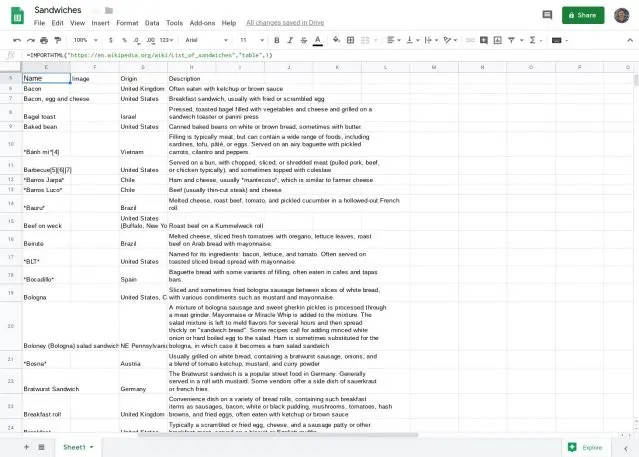
9. Sheets can pull in data from any publicly available web page, too, as long as the page has a properly formatted table. The secret lies within the ImportHTML command; use it with whatever URL you need and the number indicating which table on the page you want to import (“1” for the first table, “2” for the second, and so on):
=IMPORTHTML("https://en.wikipedia.org/wiki/List_of_sandwiches","table",1)
And just like that, all of the info will appear within your spreadsheet.
10. A similar kind of command can let you import recent entries from a website’s RSS feed into any spreadsheet. All you need to do is enter the ImportFeed command along with the URL of the feed you want—so, for instance, if you wanted to see all of my Fast Company stories in Google Sheets, you could enter:
=IMPORTFEED("https://fastcompany.com/user/jrraphael/rss")
If you wanted only the titles of the stories—and wanted only, say, the most recent five entries—you could add in the following parameters:
=IMPORTFEED("https://fastcompany.com/user/jrraphael/rss","items title",false,5)
And then if you wanted to place the links to each story in a separate column alongside that, you could use this:
=IMPORTFEED("https://fastcompany.com/user/jrraphael/rss","items URL",false,5)
11. Google Sheets has an easily overlooked cousin called Google Forms that lets you collect data in a survey-style form on the web and then compile the results in a spreadsheet. You can create a form by looking for the Form option within Sheets’ Insert menu, and then using the site that comes up to create any set of questions and parameters you want. When your form is ready, click the Send button in the upper-right corner of the page to email it to anyone, embed it in a web page, or get a manual link for sharing it however you like. As responses come in, they’ll automatically appear in your spreadsheet as their own individual rows.
Clean it up
12. If you spot some extra spaces before or after data in your spreadsheet (whether you’re looking at numbers or text), don’t forget the Google Sheets function TRIM. You can type it in for whatever cell you want, (=TRIM(A1), for instance) and it’ll take away any leading or trailing spaces and give you a cleaner version of the cell’s value.
If you want to perform the function for multiple cells at once, use this format for whatever range you need:
=ArrayFormula(TRIM(A2:A50))
13. Looking at lots of data with RanDoM or ImPropeR CaPitaLiZaTion? Sheets can standardize case formatting for you with a few simple functions: =Upper(A1) will make all of the text uppercase for whatever cell you mention; =Lower(A1) will do the same with lowercase; and =Proper(A1) will capitalize the first letter of each word for a title-case effect.
14. Maybe you have a database of user-submitted email addresses. Well, tell Sheets to look through the addresses and determine if they’re all properly formatted: Use the function IsEmail(A1) with whatever cell you need—or if you want to perform the function for a range of cells, use this format instead:
=ArrayFormula(ISEMAIL(A2:A50))
Sheets will give you a True or False answer for every email address you feed it.
15. You can validate URLs in a spreadsheet, too, to make sure you don’t have any improper items in your list. Follow the same procedure outlined in the previous tip but use the function IsURL instead.
Analyze and visualize
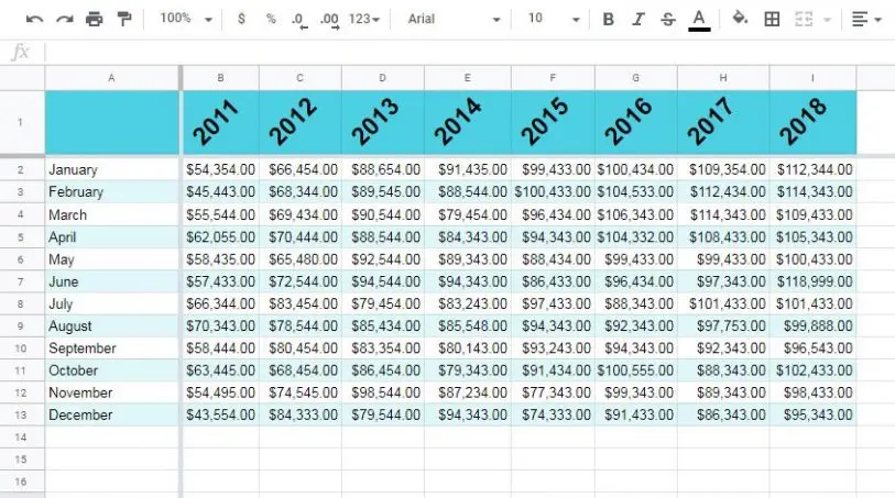
16. Perform fast calculations in any number-oriented spreadsheet by highlighting a bunch of cells and then looking in the lower-right corner of the screen. By default, Sheets will show you the sum of the numbers you’ve selected. You can then click the box with that info and tell it to show the average, the minimum or maximum, or the total count of numbers involved—and once you make that change, your selection will stick and remain the new default for any future calculations you perform.
17. Create a tiny chart within a single cell using Sheets’ nifty Sparkline feature. Just type the command =Sparkline followed by the cells you want to include, the word “charttype,” and then the type of chart you want to create—such as line, bar, or column—formatted like this:
=SPARKLINE(E12:E23,{"charttype","column"})
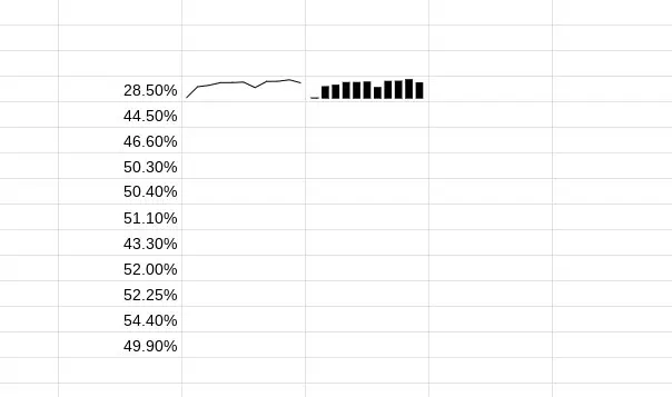
If you really want to get wild, you can even include a variety of customization commands that’ll control the colors used in different parts of your chart along with other visual factors.
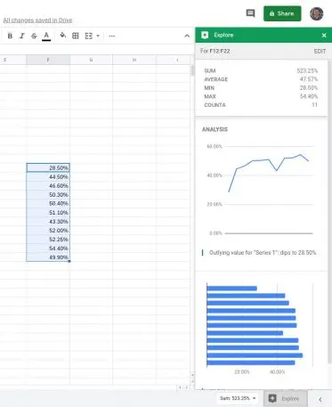
18. Tap into Google’s artificial intelligence and let Sheets perform different types of data analysis and create complex charts for you. Hover your mouse over the starburst-shaped icon in the lower-right corner of the screen, and you’ll see the word Explore appear. Click that button, and Sheets will pop up a panel of info related to your data. You can highlight specific rows in your spreadsheet to change its focus, and you can hover over any item it presents to find options for adjusting it or inserting it directly into your sheet.
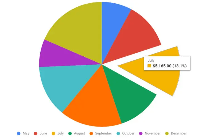
19. Sheets has a relatively new trick that can really make your pie charts pop. The next time you create a pie chart within a spreadsheet—by highlighting cells and then clicking the Insert menu followed by Chart (and then clicking Chart type to select a pie chart option, if one doesn’t come up by default)—try clicking twice on one specific piece of the pie chart and then looking for the Distance from center option in the control panel at the right side of the screen. Increase its value to 25% or more to make that segment of the chart stand out for emphasis.
Format like a pro
20. Sheets allows you to hide any row. Right-click its number in the gray column at the far left of the screen and select Hide row from the menu that appears. When you want to show the row again, click the black arrows that appeared in its place within that same left-of-screen column.
21. Want a quick and easy way to make your spreadsheet shine? Look for the Alternating colors option in Sheets’ Format menu. It’ll give you a simple set of options that’ll apply a sharp-looking color pattern to your rows—no thought or effort required.
22. While you’re jazzing up your spreadsheet’s appearance, think about letting Sheets rotate the text in your header row. Highlight the row, then click on the icon that shows an angled “A” with an up-pointing arrow beneath it (directly to the left of the link-inserting tool). You can then pick from several eye-catching effects that’ll set your header text apart and give your spreadsheet a snazzy, polished look.
23. Sheets can copy a cell’s complete set of formatting and apply it to another cell with a few fast clicks. First, click the cell with the formatting you want to copy. Then, click the paint roller icon—directly to the right of the print command, toward the left side of the toolbar—and click the cell to which you want the formatting to apply. Everything from the font size and color to the cell shading and numerical style will carry over.
24. Give yourself or your team a functional checklist right within a spreadsheet: Select a series of blank cells, open the Insert menu, and select Checkbox. You can then put your to-do items in the next column over and get the satisfaction of checking items off as you complete them.
25. Add special characters into any spreadsheet the easy way: Use the Char command and remember the numerical values of characters you frequently rely on. For instance, =CHAR(8594) will produce a right-facing arrow, =CHAR(169) will give you the copyright symbol, =CHAR(8482) will create the trademark symbol, and =CHAR(128077) will turn into the thumbs-up emoji. You can find a list of available codes on this website; just be sure to grab the numbers only (without any surrounding punctuation) from the HTML-code field.
Share and collaborate
26. Once you’ve shared a spreadsheet—either publicly or with specific people—you can create a custom link that’ll let anyone with access quickly copy your spreadsheet into their own Google account, where they can use it as a template or modify it however they want without affecting your original version. Just copy the URL in your browser’s address bar while you’re viewing the spreadsheet and replace the word “edit” at the end with “copy”—leaving you with something like this:
https://docs.google.com/spreadsheets/d/1aBcDEfgHiJKLMnOPQRSTuVWXZ/copy
When anyone with access to the spreadsheet opens that link, they’ll immediately be prompted to make a copy with a single click right then and there.
27. Sheets makes it easy to export a spreadsheet in a variety of formats via the Download as option in the File menu, but if you’d rather give people a direct link to download your data as a PDF, there’s a hidden command for doing just that: Copy your spreadsheet’s URL, just like in the previous item, but this time, replace the word “edit” at the end with “export?format=pdf”—leaving you with a link that looks something like:
https://docs.google.com/spreadsheets/d/1aBcDEfgHiJKLMnOPQRSTuVWXZ/export?format=pdf
People with access to the spreadsheet will instantly be presented with a PDF export as soon as they open the link.
28. When you’re sharing a spreadsheet or using a form to accept survey-like responses, you can ask Sheets to notify you whenever an edit or addition occurs—either immediately or as a once-daily email digest. Look for the Notification rules option in the Tools menu to set your preferences for any particular spreadsheet.
Try an advanced feature or two
29. With the help of an external service, Sheets has the capability to create QR codes that’ll pull up whatever URLs you want when they’re scanned. Type your URL into a cell (with https:// or https:// in front of it), then use the following function with your own cell number in place of “B4”:
=image("https://image-charts.com/chart?chs=150x150&cht=qr&choe=UTF-8&chl="&ENCODEURL(B4))
The QR code will instantly appear and be available to copy, share, or manipulate in any way your heart desires.

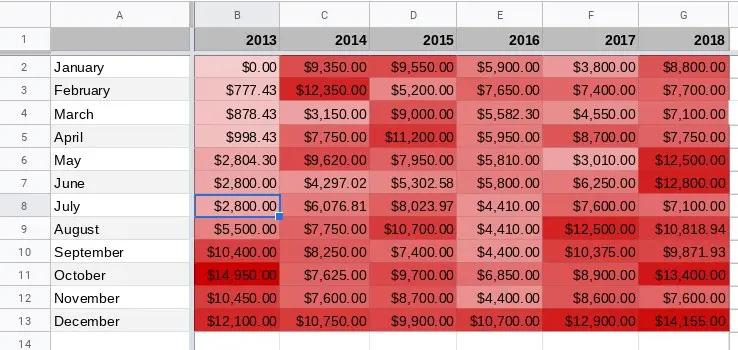
30. Here’s a handy little Sheets function for tracking trends across numerical data: Create a heat map to highlight highs and lows and make it easy to see things like sales or web-traffic success patterns. Select whatever range of data you want, then look for the Conditional formatting option within the Format menu. Click the Color scale tab at the top and assign a color to both Min value and Max value. The effect will work best if you use a light version of a color for the former and a dark version of the same color for the latter.
31. Sheets has the power of Google Finance (which—who knew?—is still a thing) baked right in for your stock-knowledge needs. The system is able to give you real-time or historical stock prices along with all sorts of other market-related data for any publicly traded company. Simply use the function GoogleFinance followed by the info you desire, using the variables and formats described on this page.
32. Ever find yourself scrolling through a list of responses in different languages? Sheets can identify any language used in a spreadsheet and even translate it into your own native tongue on the spot. To detect a language, use the following function (with the appropriate cell number in place of “A1”):
=DETECTLANGUAGE(A1)
You can also enter in a word in place of a cell number, if you want:
=DETECTLANGUAGE("queso")
Google will give you a two-letter code telling you the language that was used. To translate, meanwhile, use the following command—with your own word or cell number in place of “A1” and the code for whatever language you want to translate into (if it’s anything other than English, as referenced below):
=GOOGLETRANSLATE(A1,"auto","en")
It just goes to show you: Much like the language of love, the language of spreadsheets truly is universal.
[Editor’s note: This story was updated and expanded in May 2021.]
For even more next-level Google knowledge, check out my Android Intelligence newsletter.
Recognize your brand’s excellence by applying to this year’s Brands That Matter Awards before the early-rate deadline, May 3.
